Components

The notebook will describe the different component that can be added to the beamline, their parameters, and how to inspect the neutrons that reach each component.

import matplotlib.pyplot as plt
import numpy as np
import scipp as sc
import plopp as pp
import tof

meter = sc.Unit('m')
Hz = sc.Unit('Hz')
deg = sc.Unit('deg')

We begin by making a source pulse using the profile from ESS.

source = tof.Source(facility='ess', neutrons=1_000_000)
source.plot()

Downloading file 'ess/ess.h5' from 'https://github.com/scipp/tof-sources/raw/refs/heads/main/1/ess/ess.h5' to '/home/runner/.cache/tof'.

Adding a detector

We first add a Detector component which simply records all the neutrons that reach it. It does not block any neutrons, they all travel through the detector without being absorbed.

detector = tof.Detector(distance=30.0 * meter, name='detector')

# Build the instrument model
model = tof.Model(source=source, detectors=[detector])
model

Model:
  Source: Source:
  pulses=1, neutrons per pulse=1000000
  frequency=14.0 Hz
  facility='ess'
  distance=0.0 m
  Detectors:
    detector: Detector(name=detector, distance=30.0 m)

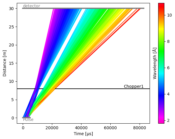
# Run and plot the rays
res = model.run()
res.plot()

Plot(ax=<Axes: xlabel='Time [μs]', ylabel='Distance [m]'>, fig=<Figure size 640x480 with 2 Axes>)

As expected, the detector sees all the neutrons from the pulse. Each component in the instrument has a .plot() method, which allows us to quickly visualize histograms of the neutron counts at the detector.

res.detectors['detector'].plot()

The data itself is available via the .toa, .wavelength, .birth_time, and .speed properties, depending on which one you wish to inspect.

print(res.detectors['detector'].toa)
print(res.detectors['detector'].wavelength)
print(res.detectors['detector'].birth_time)
print(res.detectors['detector'].speed)

toa: min=1595.5781065809065 µs, max=153334.77459370656 µs, events=1000000
wavelength: min=0.19852297909904246 Å, max=19.89582681861475 Å, events=1000000
birth_time: min=12.455804138356083 µs, max=4975.793610667868 µs, events=1000000
speed: min=198.83737640991794 m/s, max=19927.335485660773 m/s, events=1000000

Adding a chopper

Next, we add a chopper in the beamline, with a frequency, phase, distance from source, and a set of open and close angles for the cutouts in the rotating disk.

chopper1 = tof.Chopper(
    frequency=10.0 * Hz,
    open=sc.array(
        dims=['cutout'],
        values=[30.0, 50.0],
        unit='deg',
    ),
    close=sc.array(
        dims=['cutout'],
        values=[40.0, 80.0],
        unit='deg',
    ),
    phase=0.0 * deg,
    distance=8 * meter,
    name="Chopper1",
)
chopper1

Chopper(name=Chopper1, distance=8.0 m, frequency=10.0 Hz, phase=0.0 deg, direction=CLOCKWISE, cutouts=2)

We can directly set this on our existing model, and re-run the simulation.

model.add(chopper1)
res = model.run()
res.plot()

Plot(ax=<Axes: xlabel='Time [μs]', ylabel='Distance [m]'>, fig=<Figure size 640x480 with 2 Axes>)

As expected, the two openings now create two bursts of neutrons, separating the wavelengths into two groups.

If we plot the chopper data,

res.choppers['Chopper1'].toa.plot()

we notice that the chopper sees all the incoming neutrons, and blocks many of them (gray), only allowing a subset to pass through the openings (blue).

The detector now sees two peaks in its histogrammed counts:

res.detectors['detector'].toa.plot()

Multiple choppers

It is of course possible to add more than one chopper. Here we add a second one, further down the beam path, which splits each of the groups into two more groups.

chopper2 = tof.Chopper(
    frequency=5.0 * Hz,
    open=sc.array(
        dims=['cutout'],
        values=[30.0, 40.0, 55.0, 70.0],
        unit='deg',
    ),
    close=sc.array(
        dims=['cutout'],
        values=[35.0, 48.0, 65.0, 90.0],
        unit='deg',
    ),
    phase=0.0 * deg,
    distance=20 * meter,
    name="Chopper2",
)

model.add(chopper2)
res = model.run()
res.plot()

Plot(ax=<Axes: xlabel='Time [μs]', ylabel='Distance [m]'>, fig=<Figure size 640x480 with 2 Axes>)

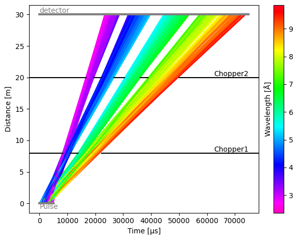
The distribution of neutrons that are blocked and pass through the second chopper looks as follows:

res.choppers['Chopper2'].plot()

while the detector now sees 4 peaks

res.detectors['detector'].plot()

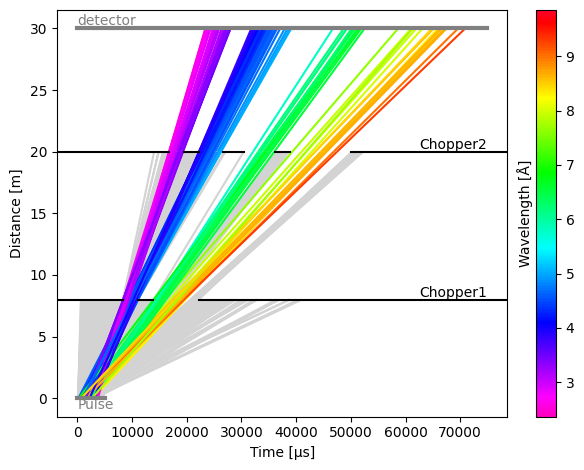
To view the blocked rays on the time-distance diagram of the model, use

res.plot(visible_rays=100, blocked_rays=5000)

Plot(ax=<Axes: xlabel='Time [μs]', ylabel='Distance [m]'>, fig=<Figure size 640x480 with 2 Axes>)

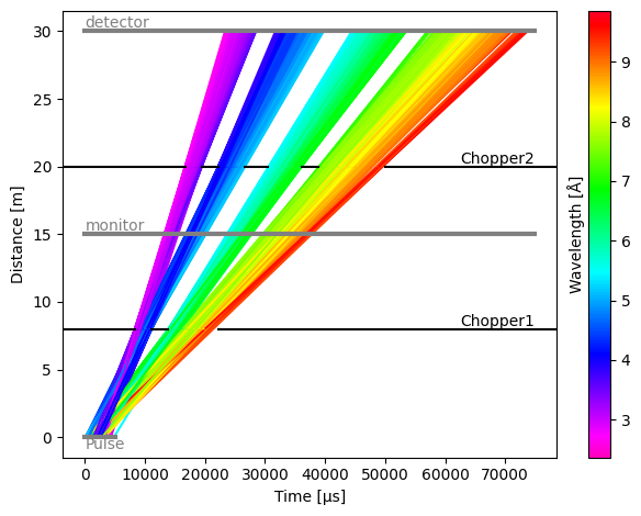
Adding a monitor

Detectors can be placed anywhere in the beam path, and in the next example we place a detector (which will act as a monitor) between the first and second chopper.

monitor = tof.Detector(distance=15.0 * meter, name='monitor')

model.add(monitor)
res = model.run()
res.plot()

Plot(ax=<Axes: xlabel='Time [μs]', ylabel='Distance [m]'>, fig=<Figure size 640x480 with 2 Axes>)

res.detectors['monitor'].plot()

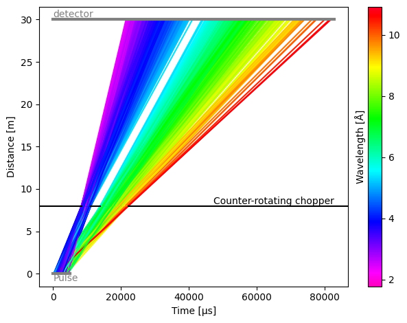
Counter-rotating chopper

By default, choppers are rotating clockwise. This means than when open and close angles of the chopper windows are defined as increasing angles in the anti-clockwise direction, the first window (with the lowest opening angles) will be the first one to pass in front of the beam.

To make a chopper rotate in the anti-clockwise direction, use the direction argument:

chopper = tof.Chopper(
    frequency=10.0 * Hz,
    open=sc.array(
        dims=['cutout'],
        values=[280.0, 320.0],
        unit='deg',
    ),
    close=sc.array(
        dims=['cutout'],
        values=[310.0, 330.0],
        unit='deg',
    ),
    direction=tof.AntiClockwise,
    phase=0.0 * deg,
    distance=8 * meter,
    name="Counter-rotating chopper",
)

model = tof.Model(source=source, detectors=[detector], choppers=[chopper])
res = model.run()

res.plot()

Plot(ax=<Axes: xlabel='Time [μs]', ylabel='Distance [m]'>, fig=<Figure size 640x480 with 2 Axes>)

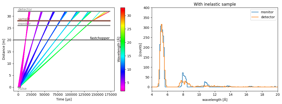
Inelastic sample

Placing an InelasticSample in the instrument will change the energy of the incoming neutrons by a \(\Delta E\) defined in a function. That function takes in the incident energy and returns the final energy after the energy transfer took place.

To give an equal chance for a random \(\Delta E\) between -0.2 and 0.2 meV, we can use Numpy’s uniform random sampling:

rng = np.random.default_rng(seed=83)


def uniform_deltae(e_i):
    # Uniform sampling between -0.2 and 0.2 meV
    de = sc.array(
        dims=e_i.dims, values=rng.uniform(-0.2, 0.2, size=e_i.shape), unit='meV'
    )
    return e_i.to(unit='meV', copy=False) - de


sample = tof.InelasticSample(
    distance=28.0 * meter, name="sample", delta_e=uniform_deltae
)
sample

InelasticSample(name=sample, distance=28.0 m)

We then make a single fast-rotating chopper with one small opening, to select a narrow wavelength range at every rotation.

We also add a monitor before the sample, and a detector after the sample so we can follow the changes in energies/wavelengths.

choppers = [
    tof.Chopper(
        frequency=70.0 * Hz,
        open=sc.array(dims=['cutout'], values=[0.0], unit='deg'),
        close=sc.array(dims=['cutout'], values=[1.0], unit='deg'),
        phase=0.0 * deg,
        distance=20.0 * meter,
        name="fastchopper",
    ),
]

detectors = [
    tof.Detector(distance=26.0 * meter, name='monitor'),
    tof.Detector(distance=32.0 * meter, name='detector'),
]

source = tof.Source(facility='ess', neutrons=5_000_000)

model = tof.Model(source=source, components=choppers + detectors + [sample])
res = model.run()


fig, ax = plt.subplots(1, 2, figsize=(12, 4.5))

dw = sc.scalar(0.1, unit='angstrom')
pp.plot(
    {
        'monitor': res['monitor'].data.hist(wavelength=dw),
        'detector': res['detector'].data.hist(wavelength=dw),
    },
    title="With inelastic sample",
    xmin=4,
    xmax=20,
    ymin=-20,
    ymax=400,
    ax=ax[1],
)

res.plot(visible_rays=10000, ax=ax[0])

Plot(ax=<Axes: xlabel='Time [μs]', ylabel='Distance [m]'>, fig=<Figure size 1200x450 with 3 Axes>)

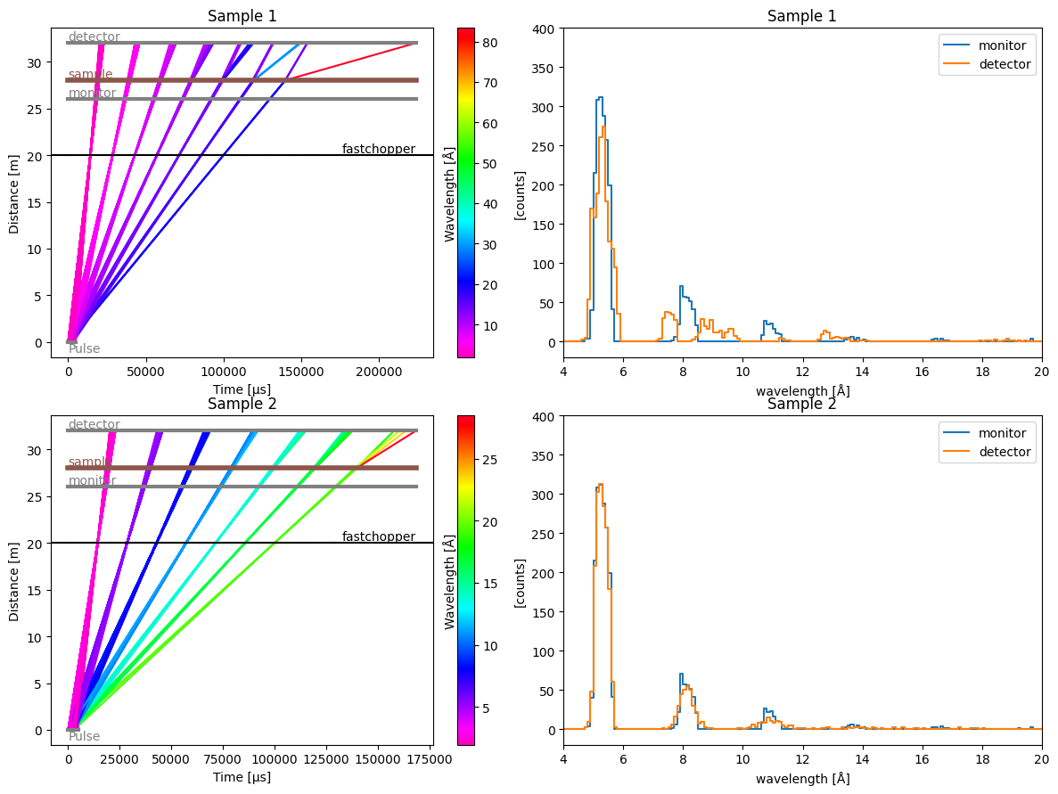
Non-uniform energy-transfer distributions

# Sample 1: double-peak at min and max
def double_peak(e_i):
    # Either -0.2 or 0.2 meV
    de = sc.array(
        dims=e_i.dims, values=rng.choice([-0.2, 0.2], size=e_i.shape), unit='meV'
    )
    return e_i.to(unit='meV', copy=False) - de


sample1 = tof.InelasticSample(
    distance=28.0 * meter,
    name="sample",
    delta_e=double_peak,
)


# Sample 2: normal distribution
def normal_deltae(e_i):
    de = sc.array(
        dims=e_i.dims, values=rng.normal(scale=0.05, size=e_i.shape), unit='meV'
    )
    return e_i.to(unit='meV', copy=False) - de


sample2 = tof.InelasticSample(
    distance=28.0 * meter,
    name="sample",
    delta_e=normal_deltae,
)

model1 = tof.Model(source=source, components=choppers + detectors + [sample1])
model2 = tof.Model(source=source, components=choppers + detectors + [sample2])

res1 = model1.run()
res2 = model2.run()

fig, ax = plt.subplots(2, 2, figsize=(12, 9))

res1.plot(visible_rays=10000, ax=ax[0, 0], title="Sample 1")
pp.plot(
    {
        'monitor': res1['monitor'].data.hist(wavelength=dw),
        'detector': res1['detector'].data.hist(wavelength=dw),
    },
    title="Sample 1",
    xmin=4,
    xmax=20,
    ymin=-20,
    ymax=400,
    ax=ax[0, 1],
)

res2.plot(visible_rays=10000, ax=ax[1, 0], title="Sample 2")
_ = pp.plot(
    {
        'monitor': res2['monitor'].data.hist(wavelength=dw),
        'detector': res2['detector'].data.hist(wavelength=dw),
    },
    title="Sample 2",
    xmin=4,
    xmax=20,
    ymin=-20,
    ymax=400,
    ax=ax[1, 1],
)

Dealing with un-physical energies

By default, a safety check is run on the final neutron energies returned by the function the user supplies to simulate the energy transfer.

It could be that the energy loss is so large that the final wavelength becomes negative, which is unphysical. The safety check simply gives these neutrons an energy close to zero (1e-30 meV).

But this may not be what the user wants. In the following example, we throw away unphysical neutrons by giving them a NaN energy.

# A DeltaE which leads to negative energies
def large_deltae(e_i):
    de = sc.array(
        dims=e_i.dims, values=rng.uniform(-0.6, 0.6, size=e_i.shape), unit='meV'
    )
    return e_i.to(unit='meV', copy=False) - de


# The same DeltaE but we throw away unphysical neutrons
def deltae_with_throwaway(e_i):
    e_f = large_deltae(e_i)
    zero_energy = sc.scalar(0.0, unit='meV')
    e_f = sc.where(e_f < zero_energy, sc.scalar(np.nan, unit='meV'), e_f)
    return e_f


res = []
for func in (large_deltae, deltae_with_throwaway):
    sample = tof.InelasticSample(distance=28.0 * meter, name="sample", delta_e=func)
    model = tof.Model(source=source, components=choppers + detectors + [sample])
    res.append(model.run())

print(res[0]['monitor'].wavelength.max(), res[0]['detector'].wavelength.nanmax())
print(res[1]['monitor'].wavelength.max(), res[1]['detector'].wavelength.nanmax())

<scipp.Variable> ()    float64             [Å]  19.6966 <scipp.Variable> ()    float64             [Å]  9.04457e+15
<scipp.Variable> ()    float64             [Å]  19.6966 <scipp.Variable> ()    float64             [Å]  34.764

We can see that in the case of large_deltae, the maximum wavelength at the detector is a very large number, while for deltae_with_throwaway the unphysical wavelengths were thrown away with NaNs and the nanmax() returns a more reasonable value.

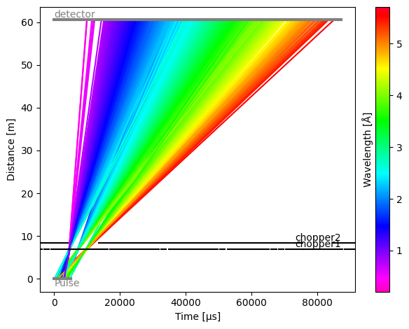
Loading components from a JSON file

It is also possible to load components from a JSON file, which can be very useful to quickly load a pre-configured instrument.

To illustrate the format, we first create a small JSON file and save it to disk:

import json

params = {
    "source": {"type": "source", "facility": "ess", "neutrons": 1e6, "pulses": 1},
    "chopper1": {
        "type": "chopper",
        "frequency": {"value": 56.0, "unit": "Hz"},
        "phase": {"value": 93.244, "unit": "deg"},
        "distance": {"value": 6.85, "unit": "m"},
        "open": {
            "value": [-1.9419, 49.5756, 98.9315, 146.2165, 191.5176, 234.9179],
            "unit": "deg",
        },
        "close": {
            "value": [1.9419, 55.7157, 107.2332, 156.5891, 203.8741, 249.1752],
            "unit": "deg",
        },
        "direction": "clockwise",
    },
    "chopper2": {
        "type": "chopper",
        "frequency": {"value": 14.0, "unit": "Hz"},
        "phase": {"value": 45.08, "unit": "deg"},
        "distance": {"value": 8.45, "unit": "m"},
        "open": {"value": [-23.6029], "unit": "deg"},
        "close": {"value": [23.6029], "unit": "deg"},
        "direction": "clockwise",
    },
    "detector": {"type": "detector", "distance": {"value": 60.5, "unit": "m"}},
}

with open("my_instrument.json", "w") as f:
    json.dump(params, f)

!head my_instrument.json

{"source": {"type": "source", "facility": "ess", "neutrons": 1000000.0, "pulses": 1}, "chopper1": {"type": "chopper", "frequency": {"value": 56.0, "unit": "Hz"}, "phase": {"value": 93.244, "unit": "deg"}, "distance": {"value": 6.85, "unit": "m"}, "open": {"value": [-1.9419, 49.5756, 98.9315, 146.2165, 191.5176, 234.9179], "unit": "deg"}, "close": {"value": [1.9419, 55.7157, 107.2332, 156.5891, 203.8741, 249.1752], "unit": "deg"}, "direction": "clockwise"}, "chopper2": {"type": "chopper", "frequency": {"value": 14.0, "unit": "Hz"}, "phase": {"value": 45.08, "unit": "deg"}, "distance": {"value": 8.45, "unit": "m"}, "open": {"value": [-23.6029], "unit": "deg"}, "close": {"value": [23.6029], "unit": "deg"}, "direction": "clockwise"}, "detector": {"type": "detector", "distance": {"value": 60.5, "unit": "m"}}}

We now use the tof.Model.from_json() method to load our instrument:

model = tof.Model.from_json("my_instrument.json")
model

Model:
  Source: Source:
  pulses=1, neutrons per pulse=1000000
  frequency=14.0 Hz
  facility='ess'
  distance=0.0 m
  Choppers:
    chopper1: Chopper(name=chopper1, distance=6.85 m, frequency=56.0 Hz, phase=93.244 deg, direction=CLOCKWISE, cutouts=6)
    chopper2: Chopper(name=chopper2, distance=8.45 m, frequency=14.0 Hz, phase=45.08 deg, direction=CLOCKWISE, cutouts=1)
  Detectors:
    detector: Detector(name=detector, distance=60.5 m)

We can see that all components have been read in correctly. We can now run the model:

model.run().plot()

Plot(ax=<Axes: xlabel='Time [μs]', ylabel='Distance [m]'>, fig=<Figure size 640x480 with 2 Axes>)

Modifying the source

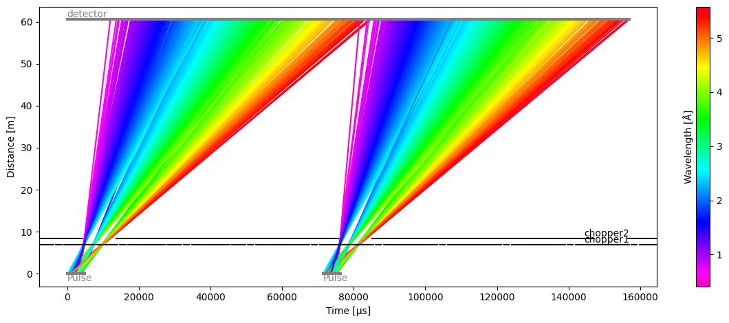
The source in the instrument JSON file may need to be tweaked or swapped out entirely for a new one. Alternatively, the source may not even be specified in the JSON file.

To place a new source inside the model, simply create one and add it to the model:

model.source = tof.Source(facility='ess', neutrons=1e4, pulses=2)

model.run().plot()

Plot(ax=<Axes: xlabel='Time [μs]', ylabel='Distance [m]'>, fig=<Figure size 1200x480 with 2 Axes>)

Saving to JSON

To share beamline parameters and models, you can save a model to a JSON file using the to_json method:

model.to_json("new_instrument.json")